Stratifying data
Stratifying groups rows by a specified number of equal intervals on a numeric column and counts the rows in each group. You can also subtotal numeric columns for each interval.
How it works
Sorting
You do not need to sort data before stratifying.
Order of operations
When you stratify data, Add-In for Excel:
- groups the rows using intervals based on the values in a numeric column
- subtotals the number of rows in each group and calculates the percentage of the total count represented by each group
- for each numeric subtotal column included in the results, subtotals each unique value and calculates the percentage of the total value represented by each subtotal
Example
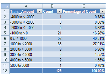
You are working with an accounts receivable table and you need to find the total number of transactions per amount interval. To find this, you stratify the data using the transaction amount column and subtotal the transaction amount column.
Outputting results to Pivot reports
If you output the results of stratifying to a PivotTable or PivotChart, you can further group the stratify intervals by the values in additional columns.
Example
You are working with an accounts receivable table and you need to find the total number of transactions per customer per amount interval. To find this, you stratify the data using the transaction amount column and then group the intervals by customer ID. You also subtotal the transaction amount column.

Stratify data
Select the stratify column
- With a cell selected in an ACL Add-In table, click the ACL Add-In tab and select Summarize > Stratify.
- Select a numeric column to stratify.
- Optional To omit the count or percentage
for the stratify intervals, clear Include
count or Include percentage.
If you clear Include count, Include percentage is also automatically cleared.
- In the Number of intervals field, enter the number of intervals that will be used for stratifying the values in the column you selected, or keep the default number of 10.
- To configure subtotals and pivot output, click Next or click Finish to output the results as is.
Select the numeric subtotal columns
- Select one or more numeric columns to subtotal.
- Optional To omit the percentage for the subtotal amounts, clear Include percentage.
- To configure pivot output, click Next or click Finish to output the results as is.
Define the output format
To define the output format, select one of the following output options and then click Finish:
- ACL Add-In Table outputs a defined ACL Add-in table
- PivotTable outputs a standard Excel PivotTable
- PivotChart outputs a standard Excel PivotChart with the accompanying PivotTable
The output results appear in a new ACL Add-In worksheet. If you output the results to a PivotTable or PivotChart, you can further group stratified intervals by additional columns, or add additional subtotal columns:
- Click any cell in the PivotTable, or click the PivotChart.
- If the Pivot Table Field List does not appear, with a cell in the PivotTable selected, click the Options tab and select Field List.
- In the PivotTable Field List, select additional columns to group intervals or subtotal on.